Variant caller benchmark

Inside daisy’s task library are some common tools used for variant calling. The following guide shows how to install daisy and run a variant-caller benchmark on publicly available data. It starts from scratch, though you will have to have installed a conda environment.

Installation

We start by creating a conda environment and installing daisy:

conda create -y -n daisy python=3.6 matplotlib
pip install cgatcore
pip install cgat-daisy
conda install ruamel_yaml pysam

Note

We use a pip install until conda packages is available and are up-to-date.

Next, we install a few variant callers (freebayes, octopus and bcftools) and variant metrics that we want to test:

conda install -y -c bioconda freebayes octopus bcftools samtools bedtools

All of these have already been wrapped in daisy’s Task Library and are ready to be used. Next, we download the aligned exome sequencing data of the NA12878. We will only use chromosome 20 to avoid downloading the whole file (26Gb):

samtools view -h ftp://ftp-trace.ncbi.nih.gov/1000genomes/ftp/technical/working/20120117_ceu_trio_b37_decoy/CEUTrio.HiSeq.WEx.b37_decoy.NA12878.clean.dedup.recal.20120117.bam 20 | samtools view -bS > NA12878.bam
samtools index NA12878.bam

For variant calling, we will also need the reference genome sequence:

wget ftp://ftp.1000genomes.ebi.ac.uk/vol1/ftp/technical/reference/phase2_reference_assembly_sequence/hs37d5.fa.gz
gunzip hs37d5.fa

Running the benchmarks

Create a benchmark.yml file:

title : >-
  Benchmarking variant callers on NA12878 exome data

description: >-
  This benchmark calls short variants on NA12878 exome data
  evaluates the results by comparison against a truth data set
  (Genomes in a Bottle, NA12878).

tags:
  - SNV calling
  - NA12878

database:
  # we will uload results to a local sqlite database
  url: sqlite:///./csvdb

setup:
  suffix: vcf.gz

  tools:
    - bcftools
    - freebayes
    - octopus

  metrics:
    - bcftools_stats

input:
  reference_fasta: hs37d5.fa

  bam:
    - NA12878.bam

bcftools:
  options: --format-fields GQ,GP --multiallelic-caller

bcftools_stats:
  options: --fasta-ref hs37d5.fa --apply-filters "PASS,."
  # apply a hard filter to freebayes output
  task_specific:
    freebayes.*:
      filter_exclude: "FORMAT/GT == '.' || INFO/DP < 5 || QUAL < 20"

Now run the benchmark:

daisy run -v 5 make all

You can now upload the results to the database:

daisy run -v 5 make upload

This will organize the metric data into an sqlite database. To get the number of variants called, you can query the database:

sqlite3 -header -csv csvdb "select i.tool_name, m.key, m.value
        FROM bcftools_stats_summary_numbers AS m, instance AS i
        WHERE i.id = m.instance_id AND key='number_of_SNPs' "

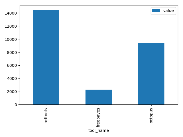
which will produce the following output:

tool_name	key	value
bcftools	number_of_SNPs	14454
freebayes	number_of_SNPs	2308
octopus	number_of_SNPs	9386

Note that such tables can be easily obtained within pandas and used for plotting. For example, the following small python snippet:

import pandas
import sqlalchemy
import matplotlib.pyplot as plt

database = sqlalchemy.create_engine("sqlite:///./csvdb")
df = pandas.read_sql(
    "SELECT i.tool_name, m.key, m.value "
    "FROM bcftools_stats_summary_numbers AS m, instance AS i "
    "WHERE i.id = m.instance_id AND key='number_of_SNPs' ", database).set_index("tool_name")

df.plot.bar()
plt.tight_layout()
plt.savefig("number_variants.png")

will create the following figure:

Adding another metric

For a proper variant caller comparison, we should compare against a gold standard of variant calls for our data set. This is available from the NIST/Genome in a bottle initiative:

wget ftp://ftp-trace.ncbi.nlm.nih.gov/giab/ftp/release/NA12878_HG001/latest/GRCh37/HG001_GRCh37_GIAB_highconf_CG-IllFB-IllGATKHC-Ion-10X-SOLID_CHROM1-X_v.3.3.2_highconf_PGandRTGphasetransfer.vcf.gz
wget ftp://ftp-trace.ncbi.nlm.nih.gov/giab/ftp/release/NA12878_HG001/latest/GRCh37/HG001_GRCh37_GIAB_highconf_CG-IllFB-IllGATKHC-Ion-10X-SOLID_CHROM1-X_v.3.3.2_highconf_PGandRTGphasetransfer.vcf.gz.tbi
wget ftp://ftp-trace.ncbi.nlm.nih.gov/giab/ftp/release/NA12878_HG001/latest/GRCh37/HG001_GRCh37_GIAB_highconf_CG-IllFB-IllGATKHC-Ion-10X-SOLID_CHROM1-X_v.3.3.2_highconf_nosomaticdel.bed

Because this is an exome data set, we restrict the high-confidence regions to captured regions:

bedtools genomecov -ibam NA12878.bam -bg | awk '$4 >= 10 ' | bedtools merge -d 10 -i stdin | bgzip > high_coverage_regions.bed.gz
bedtools intersect -a HG001_GRCh37_GIAB_highconf_CG-IllFB-IllGATKHC-Ion-10X-SOLID_CHROM1-X_v.3.3.2_highconf_nosomaticdel.bed -b high_coverage_regions.bed.gz | bedtools sort | bgzip > callable_regions.bed.gz
tabix -p bed callable_regions.bed.gz

For the comparison, we will use the vcfeval tool from RealTimeGenomics:

conda install -c bioconda rtg-tools

The toolkit requires its specially formatted reference sequence:

rtg RTG_MEM=16G format -o hs37d5.sdf hs37d5.fa

Now we can amend our benchmark.yml file by adding the rtg_vcfeval metric to the metrics section:

metrics:
  - bcftools_stats
  - rtg_vcfeval

The RTG vcfeval tool requires a bit of configuration, so we add the following to benchmark.yml:

rtg_vcfeval:
  path: rtg RTG_MEM=16G
  map_unknown_genotypes_to_reference: 1
  reference_sdf: hs37d5.sdf
  reference_vcf: HG001_GRCh37_GIAB_highconf_CG-IllFB-IllGATKHC-Ion-10X-SOLID_CHROM1-X_v.3.3.2_highconf_PGandRTGphasetransfer.vcf.gz
  callable_bed: callable_regions.bed.gz
  options: --sample=HG001,NA12878 --ref-overlap

We re-run our benchmark:

daisy run -v 5 make all

Note that the variant callers are not re-run, but only additional metrics are computed. Behind the scenes, daisy builds a ruffus workflow which means only tasks that are not up-to-date will be executed. After uploading:

daisy run -v 5 make all

We now have false positive rates and false negative rates in our table:

s3 csvdb "select i.tool_name, m.* from rtg_vcfeval AS m, instance AS i where i.id = m.instance_id "

tool_name	threshold	true_positive_baseline	true_positive_count	false_positive_count	false_negative_count	false_discovery_rate	false_negative_rate	f_measure	instance_id
bcftools	12.000	1542	1542	63	103	0.0393	0.0626	0.9489	4
bcftools	None	1544	1544	67	101	0.0416	0.0614	0.9484	4
freebayes	None	1607	1586	167	38	0.0953	0.0231	0.9394	5
octopus	5.000	1518	1518	25	127	0.0162	0.0772	0.9523	6
octopus	None	1518	1518	26	127	0.0168	0.0772	0.952	6

Next steps

The following are some advanced features not covered in this tutorial:

• Running on multiple data sets within the same benchmark.
• Aggregation of data sets, for example for trio analysis.
• Running time-series analysis for monitoring tool performance.